Law of Large Numbers and Central Limit Theorem

Sat, Mar 16, 2019 6-minute read

Many times it’s not possible to have the exact distribution of a random variable (RV), so we must estimate it. There are some tatics to approach this problem. Here, I’ll share some notes from what I’ve been studying to deal with the problem: Bound inequalities and Limit Theorems.

1. Bounds using inequalities

We have useful inequalities that help us to estimate the tail value of a probability distribution for a specific value \(a\) when the mean and the variance are easily computable, but we don’t have information about the distribution. These two inequalities usually assign a wide range value what it is not the ideal, but at least it is guaranteed that the exact answer is inside the range.

Markov Inequality

for a nonnegative random variable \(X\) and constant \(a > 0\),

\[ P(X \geq a) \leq \frac{E[X]}{a} \]

This inequality provides an upper bound for the maximum value of probability that we can expect on \(X\) to reach a value \(a\).

Loosely speaking, it asserts that if a nonnegative random variable has a small mean, then the probability that it takes a large value must also be small [1].

Chebyshev Inequality

The Chebyshev inequality follows the Markov inequality. It substitutes the RV \(X\) above by \((X - \mu)^2\), and \(a\) by \(c^2\).

\[ P(|X - \mu| \geq c) \leq \frac{\sigma^2}{c^2} \]

Loosely speaking, it asserts that when the variance of a random variable is small, the probability that it takes a value far from the mean is also small. [1]

The Chebyshev’s inequality is usually more accurate than Markov inequalities since this one uses one more information: the variance.

2. Limit Theorems

The limit theorems Law of Large Numbers (LLN) and Central Limit Theorem (CLT) help us to have an approximation of the expected value \(E[X]\) of a random variable from a large amount of data.

Law of Large Numbers (LLN)

We assume a set of RV i.i.d. \(X_1, X_2, X_3, ...\) with finite \(\mu\) and finite variance \(\sigma^2\). And define a RV sample mean \(\bar{X}_n\): \[\bar{X}_n = \frac{X_1 + ... + X_n}{n}\]

The LLN says that as \(n\) tends to infinite the \(\bar{X}_n\) converges to the true mean \(\mu\). In probability, the convergence of a RV to a number means \(P(X_n = \mu) \to 1\) as \(n \to \infty\). This statement is called the Strong Law of Large Numbers.

Also there is the Weak Law of Large Number which is easier to prove than the strong one. The weak law states that \(P(|\bar{X}_n - \mu| \geq \epsilon) \to 0\) as \(n \to \infty\). To prove this we take the Chebyshev’s inequality:

\[Var(\bar{X}_n) = \frac{Var(X)}{n} = \frac{\sigma^2}{n}\] \[P(|X_n - \mu| \geq \epsilon) \leq \frac{\sigma^2}{n\epsilon^2}\] Therefore as \(n \to \infty\), the probability goes to zero.

Central Limit Theorem

The LLN states about the sample mean convergence, but… What about the sample mean distribution ? This is addressed by the Central Limit Theorem. The CLT states that for a large \(n\), the distribution of \(\bar{X}_n\), after a standardization process, approaches the standard Normal distribution: \[Z_n = \frac{\sqrt{n}(\bar{X}_n - \mu)}{\sigma}\] The CDF of \(Z_n\) converges to the standard normal CDF \(\Phi(z)\): \[\lim_{n\to\infty} P(Z_n \leq z) = \Phi(z), \]

for every z. This can also be translated to

\[\bar{X_n} \sim \mathcal{N}(\mu, \sigma²/n)\]

No matter what is the \(X\) distribution, the sample mean process will take the Normal distribution.

An aditional information that the CLT can provides to us is our expectation of deviation from the mean, in accord with the sample size \(n\).

For example, for a Bernoulli distribution we expect the sample mean to approximate to: \[\bar{X}_n \sim \mathcal{N}\Big(\frac{1}{2}, \frac{1}{4n}\Big)\] And we know that in a Normal distribution, 95% of the distribution is around the mean by \([\mu - 2\sigma, \mu + 2\sigma]\). So when \(n = 100\), we have \(SD(\bar{X}_n) = \frac{1}{\sqrt{100}\sqrt{4}} = 0.05\), thus we can assign there’s a 95% of chance to be inside the range of \([0.4, 0.6]\).

3. R Example

Let’s do an exercise to estimate the sample mean. We are going to use 3 distributions: binomial, poisson and uniform. And we are going to visualize how the distribution of sample mean is spread as \(n\) grows.

This first code chunk only loads the packages and functions that I’ll use here.

library(tidyverse)
library(magrittr)

generate_X_n_i <- function(i, n, type) {
    if (type == "binomial") {
        X_is <-  rbinom(n, size = 10, prob = 0.5)
    } else if (type == "poisson") {
        X_is <-  rpois(n, lambda = 5)
    } else if (type == "uniform") {
        X_is <-  runif(n, max = 10)
    } else {
        stop("Choose a value to the argument \"type\" between binomial,
             poison and uniform")
    }

    mean(X_is)
}

generate_X_n_distribution <- function(sample_size, type) {
    n_simulations <- 10e3
    map_dbl(1:n_simulations, generate_X_n_i, n = sample_size, type = type)
}

plot_grid_with_distributions <- function(df, value_var) {
    df %>% 
        mutate(sample_size = factor(sample_size, levels = sample_sizes, 
                                    labels = paste0("n = ", sample_sizes)),
               type = factor(type, levels = type_distributions)) %>% 
        ggplot() +
        geom_histogram(aes(x = eval(parse(text = value_var))), bins = 100) +
        labs(x = value_var) +
        theme_bw() +
        theme(axis.title.y = element_blank(),
              axis.text.y = element_blank(),
              axis.ticks.y = element_blank(),
              axis.text.x = element_text(size = 8)) +
        facet_grid(type ~ sample_size)
}


standardize_X_n_i <- function(X_n_i, n, type) {
    if (type == "binomial") {
        mu_ <- 5
        var_ <- 5/2
    } else if (type == "poisson") {
        mu_ <- 5
        var_ <- 5
    } else if (type == "uniform") {
        mu_ <- 5
        var_ <- 100/12
    } else {
        stop("Choose a value to the argument \"type\" between binomial,
             poison and uniform")
    }
    
    (sqrt(n) * (X_n_i - mu_)) / sqrt(var_)
}

Now I plot the distributions without the standardization.

sample_sizes <- c(3, 9, 27, 81)
type_distributions  <- c("binomial", "poisson", "uniform")

df_X_n <- list(sample_size = sample_sizes, type = type_distributions) %>% 
            expand.grid(stringsAsFactors = FALSE) %>% 
            mutate(sample_mean = map2(.x = sample_size, .y = type, generate_X_n_distribution)) %$% 
            pmap_df(list(sample_size, type, sample_mean), 
                    function(x, y, z) { list(sample_size = x, type = y, sample_mean = z) %>% 
                                            as_tibble() })
    
df_X_n %>% 
    plot_grid_with_distributions(., "sample_mean")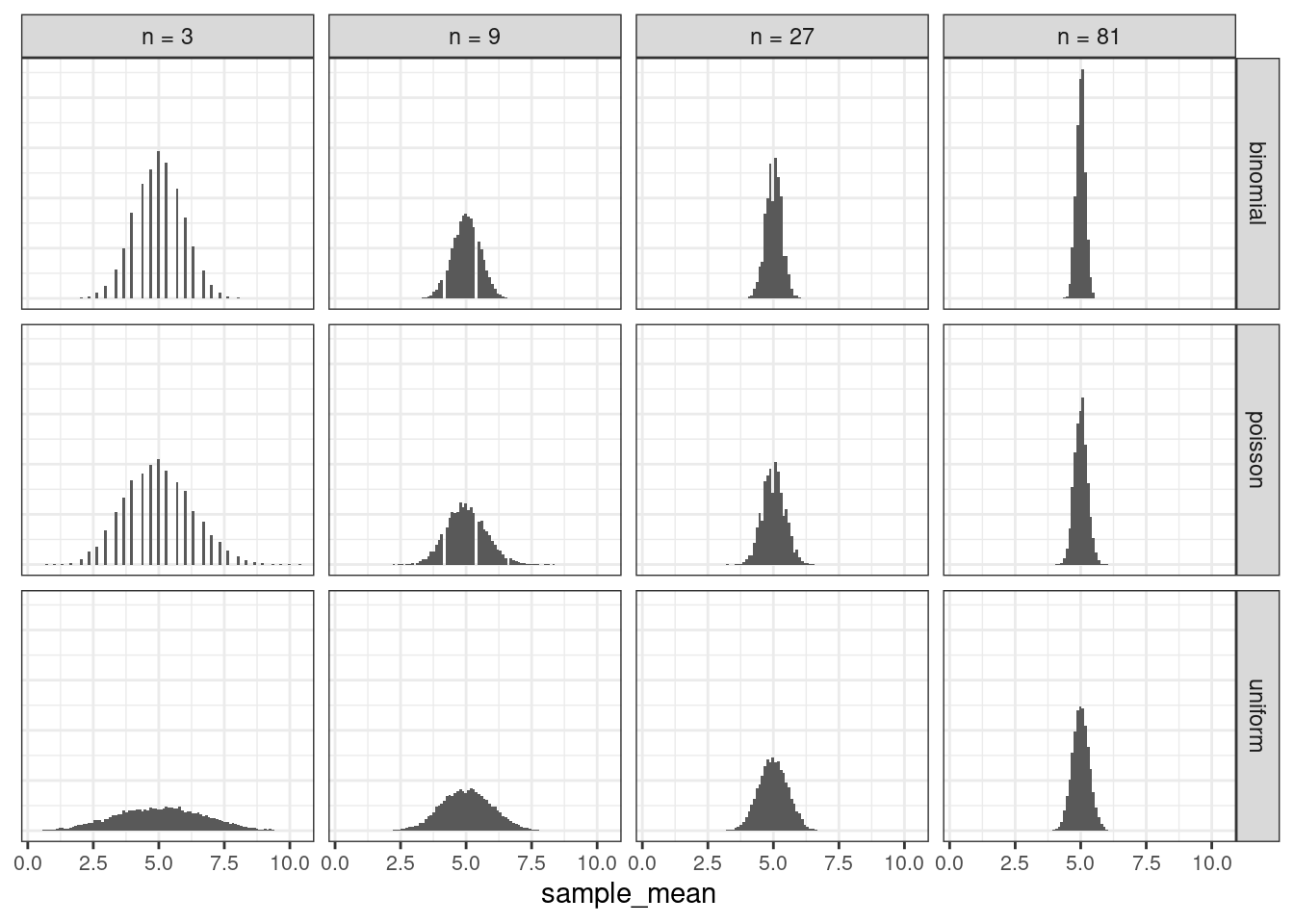

Here the bell shapes are noticed in the graphs. It also shows the LLN process, that is: the sample means are getting values in a narrow range as \(n\) grows. The variance decreases a lot.

Now we standardize it, multiplying the sample mean values by \(\sqrt{n}\) and dividing by \(\sigma\).

df_X_n %>% 
    mutate(sample_mean_standardized = pmap_dbl(list(sample_mean, sample_size, type), 
                                               standardize_X_n_i)) %>% 
    plot_grid_with_distributions(., "sample_mean_standardized")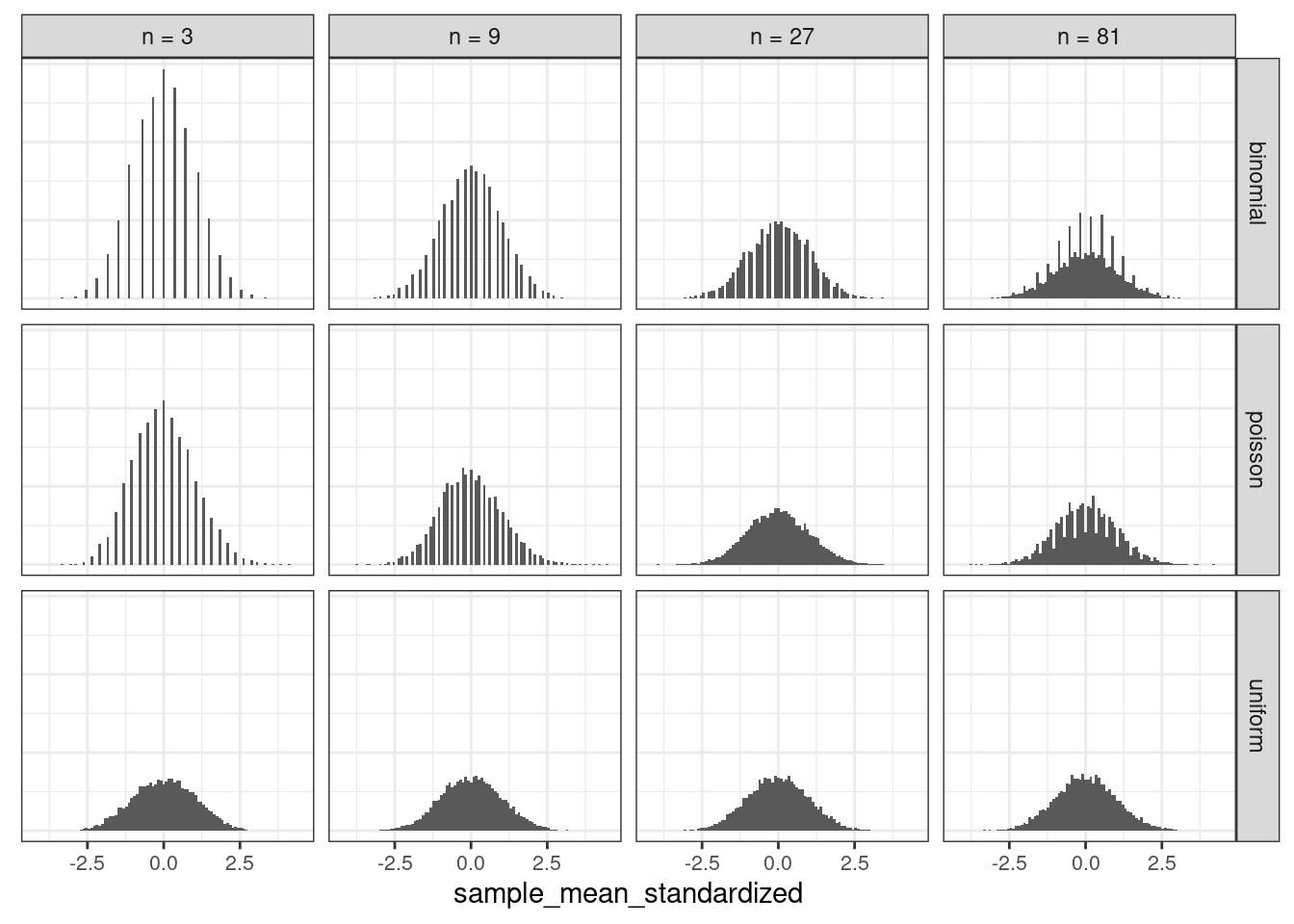

In the graph above, all distributions showed a well drawn bell shape even for small values of \(n\). Curiously, the distribution got more concentraded in few bins when \(n\) was small. It was set 100 bins in the histogram and 10 thousand simulations of sample means to all plots.

Conclusion

I could demonstrate the main points that I have seen in this interesting subject. First, how we could use information of mean and variance of a distribution to set a tail bound of probability. And how we can estimate the true mean of a population from the sample data.

Reference Material

The books:

Bertsekas, Tsitsiklis - Introduction to Probability, 2nd edition, page 382
Blitzstein, Hwang - Introduction to Probability

The authors from these books also have great lectures:

Rafael Toledo