CNN Visualizations
 |
Recently, I have played a bit with CNN visualizations and interpretability. I tried the Grad-CAM approach which extends the Class Activation Mapping (CAM) work. CAM uses global average pooling followed by a dense layer with the classes' logits as the end of the neural network; the weights assigned by each neuron’s class $c$ at each unit of the global pooling layer represent the weight of the feature map channel $k$. The pixel importance is then estimated apart for each class by the summation of weights and activation of the each channel of the feature map $M_{ij}^{c} = \sum_{k} w_{k}^{c} A_{ij}$. As the CAM method only works for the last layer, Grad-CAM estimates the $w_k$ of intermediate layers using the neuron’s gradients, such that. the $w_k^c = \frac{1}{NM} \sum_i^N \sum_j^M \frac{\partial y^c}{\partial A_{ij}^k}$
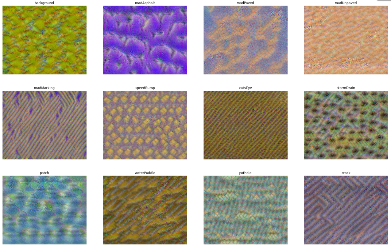
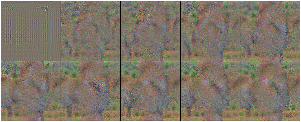
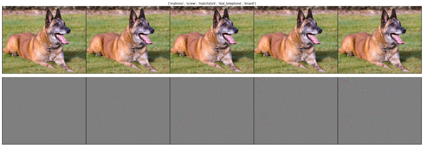
Besides estimating the region’s importance for the prediction, I tried gradient-ascent (and many regularizer tricks) to maximize the input neurons in order to have the highest output activation for a specific class. When we apply the gradient-ascent for intermediate layers' neurons, this approach leads to DeepDream. Finally, I also tried to generate adversarial examples by the reverse process of reducing the logit values of the previous predicted classes.
If you are interested in knowing more about these topics, please check the references section.
The results below are reproducible in the Colab; for more implementation details check the GitHub repo.
Semantic Segmentation
The images bellow illustrate the RTK Dataset.
GradCAM

Input Synthesis

Adversarial Examples
The rows follows the respective order: the adversarial example, the isolated noised (scaled 3x for better visualization), and the prediction results.

Classification
The images bellow illustrate the ImageNet.
GradCAM

Input Synthesis

Adversarial Examples
- The noise was scaled 10x for better visualization. The adversarial predictions were: ‘malinois’, ‘screw’, ‘matchstick’, ‘dial telephone’, and ‘briard’.

