
Deriving the Optimization Objective of Variational Autoencoder
This post intends to show how to get on the Optimization Objective of VAE, and highlights short insights about its main concepts.
Notations:
\(x\): Data or Evidence.
\(z\): Latent variables.
\(\theta\): Decoder parameters.
\(\phi\): Encoder parameters.
\(q_\phi(z|x)\): Encoder probabilistic model.
\(p_\theta(x|z)\): Decoder probabilistic model.
\(p(z)\): Prior probability distribution of \(z\).
\(z \sim q(z|x)\): the random variable \(z\) is distributed with respect to \(q(z|x)\) function.
VAE
The framework of VAE provides a computationally efficient way for optimizing Deep Latent Variable Model (DLVM) jointly with a corresponding inference model using Stochastic Gradient Descent (SGD). To turn the DLVM’s intractable posterior inference problems into tractable problems, it uses a parametric inference model \(q_{\phi}(z|x)\), which is also called an encoder or recognition model [1].
Besides the encoder, the VAE has the other coupled part, the decoder or generative model.
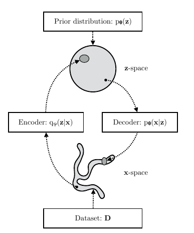
VAE diagram [1]
The Optimization Objective of VAE
The objective of the VAE is to maximize the ELBO (Evidence Lower Bound, also called Variational Lower Bound). The are some ways to derive the ELBO, the most common one is using Jensen’s inequality.
Using Jensen’s inequality
The Jensen’s inequality states \(f(\mathbb{E}[X]) \le \mathbb{E}[f(X)]\), for any convex function \(f\) as the \(\log\) function of our case.
So we can decompose the log-likelihood of the data as:
\[ \begin{aligned} \log{p_\theta(x)} &= \log{\int_{z} p_\theta(x,z) \mathrm{d}z} \\ &= \log{\int_{z} q_\phi(z|x) \frac{p_\theta(x,z)}{q_\phi(z|x)} \mathrm{d}z} \\ &= \log{\left[ \mathbb{E}_{z\sim q_\phi(z|x)}\left[ \frac{p_\theta(x,z)}{q_\phi(z|x)} \right] \right]} \\ \end{aligned} \] Applying the Jensen’s inequality on last equation, we know that: \[ \begin{aligned} \log{p_\theta(x)} &\ge \mathbb{E}_{z\sim q_\phi(z|x)}\left[ \log{\left[ \frac{p_\theta(x,z)}{q_\phi(z|x)} \right]} \right] \\ &= \mathbb{E}_{z\sim q_\phi(z|x)}\left[ \log{p_\theta(x,z)} \right] - \mathbb{E}_{z\sim q_\phi(z|x)}\left[ \log{q_\phi(z|x)} \right] \end{aligned} \]
Now decomposing the joint distribution \(p_\theta(x,z)\) to \(p(z)p_\theta(x|z)\): \[ \begin{aligned} &= \mathbb{E}_{z\sim q_\phi(z|x)}\left[ \log{p(z)} \right] + \mathbb{E}_{z\sim q_\phi(z|x)}\left[ \log{p_\theta(x|z)} \right] - \mathbb{E}_{z\sim q_\phi(z|x)}\left[ \log{q_\phi(z|x)} \right] \\ &= \mathbb{E}_{z\sim q_\phi(z|x)}\left[ \log{p_\theta(x|z)} \right] - \mathbb{E}_{z\sim q_\phi(z|x)}\left[ \log{ \frac{q_\phi(z|x)}{p(z)} } \right] \\ &= \mathbb{E}_{z\sim q_\phi(z|x)}\left[ \log{ p_\theta(x|z) } \right] - \mathcal{D}_{KL}( q_\phi(z|x) || p(z) ) \end{aligned} \]
This RHS of the equation is interpreted as the ELBO of the observed distribution. Maximizing the ELBO ensure that we maximize the log-likelihood of the observed data. \(\mathcal{D}_{KL}\) is the Kullback-Leibler divergence between two distributions, also called relative entropy.
Using an alternative approach
This method is presented on [1]. \[ \begin{aligned} \log{ p_\theta(x) } &= \mathbb{E}_{q_\phi(z|x)}\left[ \log{p_\theta(x)} \right] \\ &= \mathbb{E}_{q_\phi(z|x)}\left[ \log\left[ \frac{p_\theta(x,z)}{p_\theta(z|x)} \right] \right] \\ &= \mathbb{E}_{q_\phi(z|x)}\left[ \log\left[ \frac{p_\theta(x,z)}{q_\phi(z|x)} \frac{q_\phi(z|x)}{p_\theta(z|x)} \right] \right] \\ &= \mathbb{E}_{q_\phi(z|x)}\left[ \log\left[ \frac{p_\theta(x,z)}{q_\phi(z|x)} \right] \right] + \mathbb{E}_{q_\phi(z|x)}\left[ \log\left[ \frac{q_\phi(z|x)}{p_\theta(z|x)} \right] \right] \\ &= \mathcal{L}_{\theta, \phi}(x) + \mathcal{D}_{KL}( q_\phi(z|x) || p_\theta(z|x) ) \end{aligned} \]
The first term \(\mathcal{L_{\theta,\phi}}(x)\) is the ELBO. The second term \(\mathcal{D}_{KL}( q_\phi(z|x) || p_\theta(z|x) )\) is the relative entropy between the the approximated posterior \(q(z|x)\) and the true posterior \(p(z|x)\).
Due the non negative of Kullback-Leibler divergence, \(\mathcal{D_{KL}} \ge 0\) always. We say the ELBO is the lower bound of the log-likelihood of the data.
\[
\begin{aligned}
\mathcal{L}_{\theta, \phi}(x) &= \log{ p_\theta(x) } - \mathcal{D}_{KL}( q_\phi(z|x) || p_\theta(z|x) ) \\
&\le \log{ p_\theta(x) }
\end{aligned}
\]
Maximizing the ELBO concurrently optimize two things we care about [1]: 1. It maximizes the log-likelihood of the data \(\log{ p_\theta(x) }\), making the generative model better. 2. It minimizes the divergence between approximate posterior \(q_\phi(z|x)\) and the true posterior \(p_\theta(z|x)\), thus making \(q_\phi\) better.
Breaking the ELBO
Now, let’s get deeper decomposing the ELBO term.
\[
\begin{aligned}
L_{\theta,\phi}(x) &= \mathbb{E}_{q_\phi(z|x)}\left[ \frac{p_\theta(x,z)}{q_\phi(z|x)} \right] \\
&= \mathbb{E}_{q_\phi(z|x)}\left[ p_\theta(x|z) \frac{p(z)}{q_\phi(z|x)} \right] \\
&= \mathbb{E}_{q_\phi(z|x)}\left[ p_\theta(x|z) \right] + \mathbb{E}_{q_\phi(z|x)}\left[ \frac{p(z)}{q_\phi(z|x)} \right] \\
&= \mathbb{E}_{q_\phi(z|x)}\left[ p_\theta(x|z) \right] - \mathcal{D}_{KL}( q_\phi(z|x)||p(z) )
\end{aligned}
\]
The first term \(E_{q_\phi(z|x)}[p_\theta(x|z)]\) relates to the input data reconstruction. The second term, the KL divergence, measures the dissimilarity between the approximated posterior and the prior of \(z\).
Looking for maximizing the ELBO:
\[\theta^\*, \phi^\* = \underset{\theta,\phi}{\mathrm{argmax}} \sum_{i=1}^{N} \mathcal{L}(x^{(i)},\theta, \phi)\]
We want to maximize the likelihood of the reconstructed input, or minimize the reconstruction error, and reduce the divergence between the prior and posterior of \(z\).
References
[1] Kingma, D. P., & Welling, M. (2019). An Introduction to Variational Autoencoders. Foundations and Trends® in Machine Learning, 12(4), 307-392.